The Ultimate Guide to Multifamily Value-Add Underwriting
The Tactica Multifamily Value-Add Underwriting Guide serves three purposes:
A Tutorial - A collection of blog posts, images, videos, and links for users using the Tactica Value-Add Model. Every facet of the Excel spreadsheet is explained and can be easily navigated with the hyperlinked table of contents below.
A Preview - For viewers who need a multifamily value-add underwriting template, this blog post will detail our multifamily value-add spreadsheet, and you can determine if it’s a good fit for your business.
Knowledge - Regardless of your interest in an underwriting tool, this article provides deep insight into how to underwrite a multifamily value-add property.
Underwriting Multifamily Properties
Analyzing and underwriting a multifamily property has a lot of moving pieces. Once you possess and review the property rent roll, historical operating statements, and property tax bills, you’ll need a place to harness all this data and make investment assumptions. The key to proficient multifamily underwriting is to have a tool that you can intuitively input external data into, make your assumptions, review the results (in the form of investment returns), and stress the best and worst-case scenarios.
Value-Add Real Estate Investment Underwriting
Pre-Analysis Requirements
Enable Macros
As the workbook opens, Excel will prompt you with a yellow warning bar at the top of the screen to “Enable Macros.” Click “Enable Content.”
If you don't see this bar pop up, you can follow these steps:
File > Options > Trust Center > Trust Center Settings > Macro Settings > Enable Macros
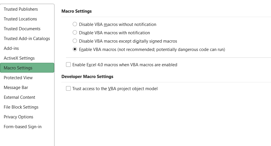
Click Ok. Save the workbook on your computer, and then close it. Once you reopen it, macros will work.
In all of the Tactica tools, all brown text cells are your responsibility. Black text hosts formulas that you should not overwrite.

Pre-Analysis Video Tutorial
Investment Summary
This tab serves two significant purposes. It is where you make the majority of your assumptions and also serves as a dashboard that can be printed and emailed to partners and investors. The dashboard will display and summarize various other components found in different tabs. The hope is that by spending five minutes on this tab, you can formulate a solid understanding of the investment viability of a particular multifamily asset.
General Property Info
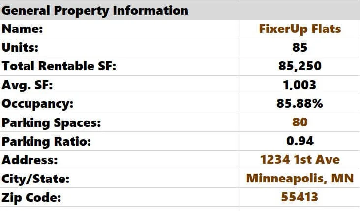
Start by keying all the general property details. About half of the cells in this section will populate from the data inputted on other tabs.
Picture of Property
This is where you can import a picture of the property or a map of its location. It’s pretty self-explanatory.
Unit Mix Summary
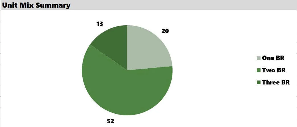
This pie chart is a simple summary of the unit mix of the apartment complex. You can update this graphic on the "Charts" tab. It is a dynamic pie chart, meaning it will update automatically as soon as you enter the unit mix on the chart tab. It should be easy to copy and paste the floor plans from the "Renovations" tab into this section. I, however, was very detailed on the Renovations tab, breaking out not only bedrooms and bathrooms but also renovated vs. original. I wanted the pie chart to be more elementary, so I took 10 seconds to type the breakout of One BR, Two BR, and Three BR units on the "Chart" tab.
Financing
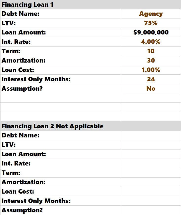
You need to input your financing terms on this page. The model supports two different loans.
An everyday use for the “Financing Loan 2” option is when a supplemental loan is involved or less expected when there is a 2nd position seller mortgage.
If you are assuming a loan, you can select "Yes" in the last row, and the model will ask you to enter what month you will be taking over the loan.
Note: The model accounts for a scenario where you assume a loan still has I/O left. Always enter the original loan terms (not just what remains for you). If you were assuming a ten-year loan that has 36 months of IO initially, and you were assuming the loan in month 25, you would input this:
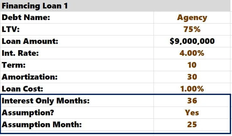
The model would know that 12 months of I/O are left when you take over ownership.
Loan #2 Creatively: A customer recently showed me how to use the Loan #2 assumption to account for a preferred equity arrangement.
Monthly payments will be calculated and stored automatically for both “free and clear” assumption scenarios on the "Debt" tab. This tab will be reviewed later.
If you don't need the second financing option, select "No" off to the right, and the Loan 2 section will remain blank. Note on top that it is "Not Applicable."
The Financing Section defaults to a Loan-To-Value (LTV) financing scenario. If you want to adjust the model flawlessly to factor in a Loan-to-Cost (LTC) scenario, you can learn how to create an LTV/LTC toggle.
Summary of Rents

A pivot table populates this chart on the "Charts" tab. This pivot table hosts the unit mix and rental information you entered on the "Renovations" tab. If you adjust floorplans, rents, or premiums on the "Renovation" tab, you must right-click the pivot table hosted on the "Charts" tab and refresh. Every time you open the workbook, pivot tables will update automatically.
If you are working on a property that doesn't have a premium upside, you can delete the "Premium" label in the chart key.
Renovation Plan

The following section is a summary of the renovation plan. This data is all pulled directly from the "Renovations" tab. The graphic on the right shows you the overview of GPR the year after the renovations are completed. Astute investors would likely do a quick cap rate calculation on the annual premium revenue to approximate how much value could be created by a successful value-add strategy.
Note: This model is also helpful if you are underwriting a Class A investment opportunity or turnkey project with little to no upside.
Cash Flow Summary
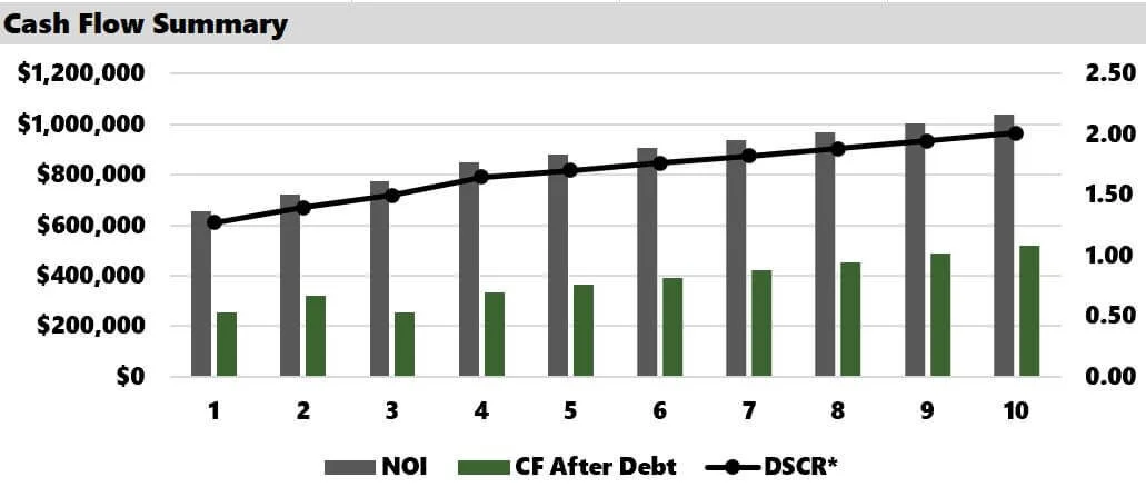
This is the final chart used on the "Summary" tab. It is meant to provide a nice visual of NOI, CF after Debt and debt service coverage ratio (DSCR) over a theoretical 10-year hold. The DSCR is always calculated based on a principal and interest payment regardless of an interest-only period.
Sources & Uses
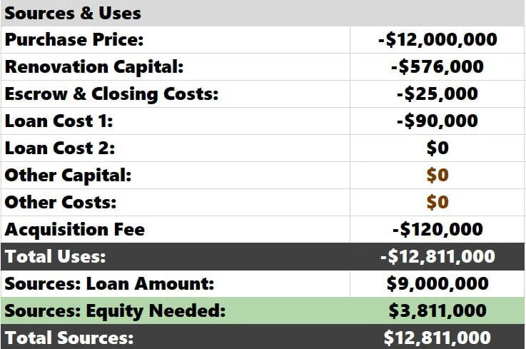
This section summarizes all costs that will encumber the investment opportunity and how it will be funded (via debt and equity). There are two cells, "Other Capital" and "Other Costs," where you can enter any additional costs you must factor in. Users will commonly use "Other Capital" for common area renovations. Enter Additional charges as negative amounts.
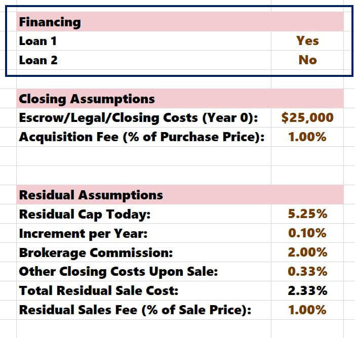
"Escrow & Closing Costs" and "Acquisition Fee" assumptions are made off to the right, outside of the view of the dashboard frame:

Project Level Metrics
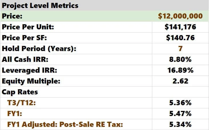
This section hosts arguably the two most essential toggles of the analysis—the purchase price and investment hold period.
You can see in real-time how various pricing metrics are affected by a change in cost and hold. The model calculates different cap rates, and you can select via a dropdown list what cap rates you want to be displayed. Real estate tax adjustments after purchase can have a massive impact on NOI. Shrewd investors always want to understand "Tax-Adjusted" cap rates on the historical and proforma NOI.
Residual Assumptions

Estimating the residual sales value is a crucial aspect of any real estate project. This data is summarized here. You will be able to see the reversion pricing metrics along with the appreciation that has taken place over the hold period. The back-end sales price is determined by the residual cap rate, which is a manual input you will make off to the right:
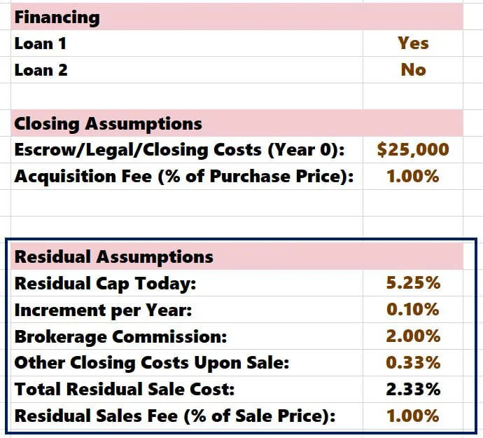
You would enter the residual cap rate today and what you expect to increase annually. In this example, if you think the cap rate is 5.25% and will grow at 0.10% annually in seven years, the residual cap rate would be 5.95% (5.25% + 0.10%*7).
You can learn more about our methodology for calculating residual sale proceeds.
You will also be responsible for entering a brokerage commission and other closing costs (as a percentage of sales price). If you are syndicating equity and charge a residual sales fee, you would also enter that amount in his section.
The Loan Paydown, Sale Costs, and Residual Sales Fee are all summarized as negative numbers, and the total sales proceeds are totaled at the bottom.
Partnership Returns

Finally, the value-add model has five different partnership structures built in. You can select which one you want to use from the drop-down list, and the model will summarize both GP and LP investment return metrics. It's important to note that the GP's IRR and equity multiple do not include any income from asset management, acquisition fees, or residual sales fees.
All partnership distribution models are linked to the hold period set on this tab. While you can change the hold period for each scenario, linking back to this tab is essential so the graphs are accurate. There is an error check to help you with this.

I would also recommend checking out how to maximize Excel’s Goal Seek analysis tool. Understanding goal seek and unleashing its potential on this tab could help you unlock solutions that may have gone unnoticed and ultimately give you ideas to persuade investors, convince lenders, or negotiate with a seller.
Renovations
The renovation model will take your analysis to a different level. The first step is to enter all the rent roll inputs. These entries include:
Unit Types (or floorplans)
Unit Count
Avg. SF
Avg. Rent
Premium
Capital Spend
Once entered, rent per square foot (PSF), Targeted rent, and Targeted Rent PSF will auto-calculate.

In this example, you can see that 13 units (15% of the units) were previously renovated, as denoted by the "R" in the Unit Type column. That's why they are not getting a premium, nor will there be any capital spent on them. The model allows up to 63 unique floor plans. I just hid the rows that I am not using.
Next, you need to define your strategy, define the timeframe, and make a vacancy assumption.

Type: Your options are:
Value-Add
Core Plus
Upside.
Value-Add is most common, "Core Plus" will be used for newer buildings that need light cosmetic upgrades, and "Upside" would be a situation where you can raise the rents without spending any money. Your designation here won't affect any calculations, just labeling.
Reno Start Year: Which year do you plan on starting the renovation? There may be instances where it would make sense to hold off until the 1st or 2nd year of the investment hold.
Years to Accomplish: How many years would it take to renovate 72 units (remember, 13 units have already been renovated in this example)? The timeframe will determine how many renovations you can accomplish each month. You must enter an integer for this assumption. Fractional years will not work (1.5 or 3.75, for example).
Month(s) Vacant: How many months will a renovated unit be vacant? One month is standard. Vacant months will affect the "Vacancy Loss Renovation" line item in the proforma. It will also affect how quickly the premium upside gets phased into the proforma. In this case, if you renovated two units per month, holding each unit vacant for one month, the premium income FY1 would be 45.83% of the total potential premium amount.
Note: This tends to confuse many people. From an underwriting perspective, renovation premiums are paid in arrears because it takes time for the upside to hit the financials. Think of buying a property and instantly renovating one unit the day you take over. Assuming one month to renovate and rent out, you would only see 91.67% of the total premium upside (or 11 out of 12 months) during Year 1.
Then, you renovate another unit the following month. You would only benefit from 10 months of premium out of 12 months. In the last month of the year, you would renovate a unit and wouldn't see any upside until next year (0 out of 12 months).
The aggregate total of this phenomenon is 45.83%, as depicted in the image above. The silver lining is that once you have completed all renovations, you will see an additional rent bump the following year, which accounts for a full 12/12 months of premium upside fully phased in. That premium upside after the renovation is complete is 54.17%.
A matrix in the financial model on the “Renovations tab” shows how the premium in arrears would calculate holding units vacant for 0.50, 1.00, 1.50, or 2.00 months.
Renovation Logic
The model will show you an excellent summary of your renovation plan:

I want to explain my renovation logic to you briefly. When you run a value-add proforma, rent growth will come from two different places.
1. The rental premiums
2. Organically, which would happen regardless of the value-add (I refer to this as "baseline rent growth").
The model allows you to control both variables. You already entered the premium but can also control the baseline rent growth.

Often, deals will have value-add potential but are under-rented even in the unit's current state. It may be necessary to increase the baseline rent by 5% and then phase the premium.
For simplicity, let's use round numbers. Let's say a 2 BR unit rents at $1,000. If you thought the unit could rent at $1,050 without renovations, you would use the grid above to increase the rent FY1 by 5%. If you thought that rehabbing the unit could create an additional $150 in premium, the logic is the following:
$1,000 * (1.05) = $1,050 = True Market Rent in Current State
$1,050 + $150 = $1,200 = True Market Rent After Renovation
The model will always increase the baseline rents per the above grid and then phase the renovation premium on top.
The final piece of the renovation analysis is to understand the results. Specifically, how do the above rents translate to annualized rent flowing into the proforma?
Renovation Results

The analysis breaks down the average rents at the property on a per-unit basis and then rolls up into the annualized Gross Potential Rent (GPR).
The model grows the baseline rents by whatever growth rates you select; the premium phases are on top of that. It's important to note that once the premium phases in, it will increase annually at whatever the baseline rent growth assumption is for that floorplan. That is the purpose of the "Total Premium Growth" line.
The capital spend/unit and renovation vacancy are summarized below. Off to the right, you can explain the renovation plan if this is something that you want to share with investors.
All this data will flow into the pro forma cash flows.
Blog Posts That Emphasize the “Renovations” Tab:
Underwriting Apartment Buildings During a Recession
Multifamily Renovation: Planning a Deeper Value-Add
Mixed-Used Proforma Underwriting Guide
Bonus: Check out the hyperlinked articles if you can add more units in a common area or combine smaller units to re-rent them as one large unit. They will touch on the Value-Add Model in the middle of each article.
Real Estate Taxes
The property tax calendar will vary from state to state. That is okay, though, because aside from slight nuances in different taxing jurisdictions, there are two crucial things that you must account for as an investor.
How much reassessment risk is there?
Which year will this reassessment risk hit the proforma?
There is a process you should follow when underwriting property taxes, and I have a separate article that serves as a guide to underwriting multifamily property tax.
I also dedicated an article to properly underwriting instances where the property tax calendar doesn't align perfectly with the proforma investment calendar. The timing of the sale can impact how you underwrite the proforma property tax. For states with multiple tax payments due throughout the year, it is crucial to understand tax "staggering" and how to use it to depict real estate tax exposure accurately.
Finally, evaluating property tax comps may be necessary when estimating your projected proforma real estate tax expense.
Financials
You'll make assumptions for other revenue line items and expenses in this tab. This tab is broken down into three parts:
Historical Financials
Proforma Assumptions
Proforma Cash Flows
Historical Financials
This tab is where you will enter the historical profit and loss data from the property (P&L).
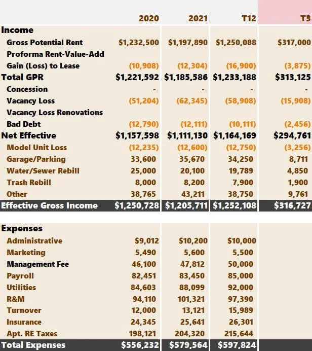
Again, all brown and orange (for the negative numbers) are your responsibility. Hopefully, you were provided the current Trailing 12 Month Financials (T12) broken down monthly and the prior two years of financial information. If this is not the case, you can hide or delete unnecessary columns. For example, if no 2020 operating information were available, I would likely hide that column so it didn't distract me.
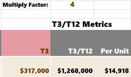
The Trailing Three (T3) Header is tinted pink, so you know to enter only three months of data. You could do a “T6”, a “T2”, or your preferred viewpoint. Just ensure you update the header and enter the corresponding months' worth of data. A “multiply factor” cell is above the “T3/T12” column. If you enter “T3,” the model will know to multiply by 4 to annualize the data. If you were going off of a T6, the model would know to multiply by 2.
The process will be slightly different if you're underwriting a pre-stabilized project.
This is a brown cell because it technically can be overwritten. The cell does, however, have a formula.
You can delete any unnecessary rows. I hide them, but removing them is fine and will not affect any calculations adversely.
After you key the historical data, you can see the annualized T3/T12 broken down in a few different ways. Many investors love breaking down line items on a "per unit" basis. I am one of them. Looking at revenue items as a % of GPR is helpful. Looking at expense items as a % of EGI is common, especially for Management Fees.

The green columns show the year-over-year historical trends. Historical EGI has been all over the place, which has caused the NOI to fluctuate wildly. The RUBS recovery shows that only 30% of the total utility expense is captured. The owner is doing okay at collecting water/sewer and trash. Is there a potential to rebill residents for Gas (heat)? What are other properties doing in the submarket? RUBS could be an area of upside.
Proforma Assumptions
Now, it's time to enter your proforma assumptions. Let's start with Year 1 (FY1).
Year 1 Assumptions
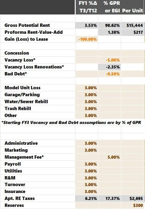
For each line item, the model allows three underwriting assumption options. You can make your assumption by:
Column 1: Increasing/Decreasing as % over the latest historical amount (T3/T12 amount in this case)
Column 2: As a % of GPR for revenue and as a % of EGI for expenses
Column 3: Per unit
With Gross Potential Rent (GPR) for both baseline rent and premiums, the assumptions have already been made on the renovations tab. The gray cells indicate that you don't need to do anything. Value-add information flows from the renovations tab, so there is nothing to do here.
I always decrease loss-to-lease by 100% in Year 1 because I will always forecast the rents based on the actual rents in place. I ignore market rents. I recommend others do the same. Concession underwriting can have a few different courses of action.
Year 2 Assumptions

Again, you can make assumptions by:
Column 1: Increasing/decreasing as % over the FY1 amounts
Column 2: As a % of GPR for revenue and as a % of EGI for expenses
Column 3: Per unit
My assumptions are similar to the ones I made in Forecast Year 1 (FY1). Reserves will continue to be $300 per unit each year.
Note: Excel will read the assumptions from left to right. Look at the administrative expenses assumptions. If I entered:
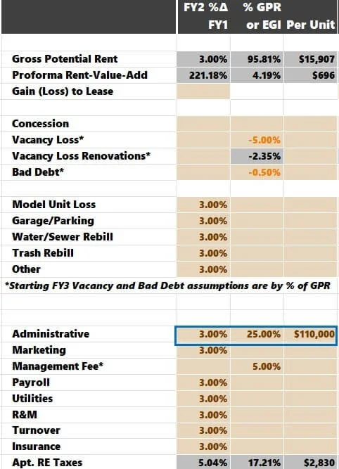
Excel would use the 3% growth over FY1, ignoring 25% and $110,000. For clarity, ensure you only have one assumption entered for each line item (excluding gray cells, which are calculated automatically).
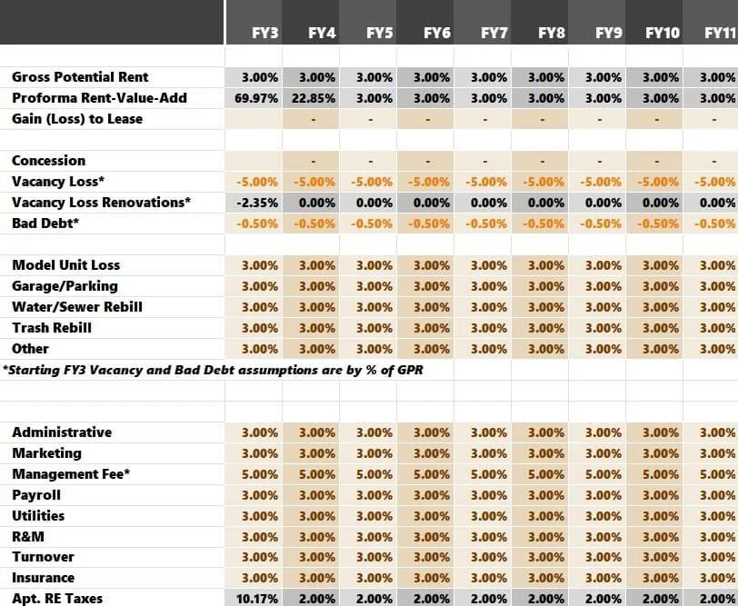
Year 3+ Assumptions
After FY2, the Years 3-11 assumption will be much more inflexible. Every line item except for Vacancy Loss, Bad Debt, and Management Fee is made as a percentage increase (or decrease) over the prior year. Vacancy and Bad Debt assumptions are a percentage of GPR. Management Fee will be a percentage of EGI. This approach is noted in the model, so you do not forget.
Proforma Cashflows
After all, you enter all assumptions; you can take a look at the cash flows off to the right:

Returns Summary
The Returns Summary is all about analyzing the numbers and calculating the return metrics. This tab will summarize the following:
Cap Rates (historical, proforma, and tax-adjusted)
All Cash Returns
IRRs and Equity multiples are calculated on various holding periods. For example, a 7-year hold would produce a Leveraged IRR of 16.69%. A 10-year hold would have a Leveraged IRR of 15.65%.
The All Cash IRR and All Cash Returns are standard metrics to analyze because they show you how the investment would look if you didn't utilize debt. It's crucial to compare the Leveraged vs. All Cash metrics to ensure that the debt is accretive and boosts your yields. In many cases, deals are over-leveraged and don't lift the returns much but exponentially take more risk.
You will need to make a couple of assumptions on this tab.
Capital Contingencies: How much capital will be paid for out of the cash flow, and over which years will it span? This assumption accounts for money you didn't raise on the front end. Think of it as a safety net.
Asset Management: If you plan on charging an asset management fee (as a percentage of EGI), you make that assumption here.
This tab is more visual in nature and is where I spend much time trying to figure out if a deal makes sense. If you downloaded the Free Multifam ly Template, the presentation on this tab is identical to the “Valuation” tab.
Additional Application: Convert an underwriting template into a hybrid analysis that factors actual historical financial performance and updated future forecasts for optimal 'hold vs. sell' decision-making
Debts
The “Debt” tab hosts the amortization tables and cash flows for the debt assumptions.
This tab doesn't require you to do anything. It is a necessary worksheet because it allows you to seamlessly toggle different debt variables such as interest-only months, amortization, “free and clear” vs. “assumption,” etc.
Charts
This tab hosts the charts presented on the "Summary" tab dashboard. You need to enter the unit mix for chart #1 and refresh the pivot table for chart #2. You can copy and paste the unit type and unit count from the "Renovation" tab to populate chart #1 as a refresher. In this example, I didn't want the unit mix pie chart on the "Summary" tab to be as detailed as what I inputted on the "Renovations" tab, so I simplified it. Regarding the pivot table for Chart #2, you only need to refresh it if you edit the inputs on the "Renovations" tab. This table will refresh automatically upon opening up the workbook.
The data for charts #3 and #4 will not need to be altered or amended.
IRR Sources
IRR is a prevalent return metric for investors to gauge the upside of an investment opportunity. What many don't realize is that the IRR is compromised of five sources:
Initial Investment Recovery
Year 1 Cash Flow
Cash Flow Increases (year-over-year)
Appreciation
Principal Loan Balance Reduction
The Tactica value-add model measures the allocation of each source. The more deals you are underwriting, the better feel you will gain for risk/reward correlation with the distribution off IRR.
Check out the article, Properly Analyzing the IRR in Real Estate Investing, to better understand how the IRR works and how you should look at it for your investments.
Renovations Stress Test
One of the favorite features for users has been the ability to stress test the renovation assumptions. Holding everything else constant, how would returns look if the rental premium is better than expected? What if the capital expense is more than initially budgeted? What if the renovation takes longer than expected? The link will take you to a written tutorial explaining the Tactica renovation stress test. Don’t forget to check out the video tutorial at the bottom of the article.
Partnership Distributions
The final step in value-add underwriting is determining the partnership distribution structure. In other words, what will the cash distribution be split between GP and LP investors? Five different options are built into the Tactica financial model.
Pari Passu
Profit Interest
Preferred Return + Profit Interest
Equity Multiple + Sale Kicker
I got into great depth, explaining each partnership distribution option in a separate blog post.
Video: Underwriting a 40-Unit Multifamily Value-Add Deal
Excel Resources
If you're interested in the inner workings of this tool to maximize its utility with advanced Excel knowledge, we recommend visiting these articles:
We plan to publish more posts about the commonly used Excel functions and the major analysis components within the Tactica models.
Summarizing Multifamily Value-Add Underwriting
This page will be updated in real-time with text, images, videos, and links explaining the new facets as updates continue to be implemented. If you purchase the value-add model, I will email you when new versions are released. If you are ever confused about something, I recommend checking here to see if your doubt can be resolved.
If you are looking for a new financial model but are not ready to commit, I recommend checking out our Free Multifamily Underwriting Template. It shares many of the same capabilities as the paid Value-Add version and will give you a good feel for the paid tools. You can register below to receive the free version.
I recommend downloading our free “back the envelope” multifamily analysis template. It is a simple one-page format to quickly vet projects before doing a more thorough underwriting analysis.